Understanding and applying oscilloscope measurements

One of the best things about digital oscilloscopes is that they can measure the acquired waveforms using a wide range of helpful measurement parameters. Most current oscilloscopes include about twenty-five standard measurement parameters with additional parameters available in application specific options. Measurements are based on a variety of industry accepted standards and produce very accurate results. A knowledge of basic measurement techniques will help oscilloscope users make the best use of measurement parameters and their related tools. This article will provide the necessary background on oscilloscope measurements and some insight into common applications.

Let’s start with basic time related measurements—period, frequency, width, and duty cycle. All these measurements are related to the time duration of various segments of a waveform and are generally applied to periodic waveforms. Figure 1 shows the basic definitions of time related measurement parameters.

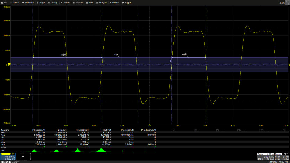
Figure 1 Time parameters are based on points where the waveform crosses a preset threshold, 50% of the waveform amplitude or zero volts in this instance. Source: Arthur Pini

Advancements in LED Drivers for Next-Generation Automotive Exterior Lighting09.18.2023

Reducing the Production Cost of Integrated Circuits in the Integration Era09.14.2023

Democratizing Edge AI and ML with a No Code Approach09.12.2023

A waveform’s period is the most basic measurement. It is the time duration on a single cycle of a periodic waveform shown as parameter P1 in the figure. The oscilloscope measures period by measuring the time between waveform crossings of a fixed threshold voltage for waveform segments with the same slope. The threshold is normally at 50% of the waveform’s amplitude but can be adjusted by the user. Period is the time per cycle. The reciprocal of the period, or cycles per unit time, is the waveform’s frequency, shown as parameter P2.

The width of a waveform is the time between threshold crossing of waveform segments with opposite slopes. If the width is measured between a positive and a negative slope it is termed positive width. The width measured between a negative and a positive slope is called the negative width. Positive width is displayed as parameter P3.

The ratio of positive width to period is defined as duty cycle and is usually expected as a percentage, reported as seen in parameter P4. Two other parameters are shown, the number of cycles and the number of edges, shown as parameters P5 and P6, respectively.

In the oscilloscope used in this example, the timing related parameters are “all instance” measurements. This means that a period value is generated for each cycle of the waveform and accumulated over multiple acquisitions. These measured values are stored and form the basis for statistical analysis, shown in the parameter readouts in the figure. The display of parameter statistics is controlled by the ‘Statistics’ check box in the measurement setup. Parameters statistics include six readout fields. For the period readout, P1, the value field shows the last measurement value accumulated. Beneath that is the mean or average value of the parameter over the total number of measurements made. The next readouts are for the minimum and maximum values encountered over the total number of measurements. The next row contains the standard deviation of the accumulated measurements. The standard deviation is a measure of the spread of the measured values about the mean value, the lower the standard deviation the more closely spaced the values. The last readout row contains the total number of measurements included in the statistics.

The status row Indicates the condition of the parameter calculation. The green check mark indicates that there are no problems with the computation.

Let’s consider a practical issue, because these parameters are based on a threshold crossing, they are prone to errors due to additive noise on the waveform. A noise peak would make the threshold crossing appear to have come earlier than expected and a noise valley would make it later. The extremes of these measurements are reported in the min and max fields as 4.9815 ns and 5.0154 ns respectively, a difference of 33.9 ps. This is the range of the measurement. The average value of the period, taken over 71,850 cycles, is reported in the mean field as 4.999993 ns. This is the best estimate of the parameter’s value in the presence of noise.

The green graphs below the parameter readouts are called ‘Histicons’, they are iconic views of the histogram of a measured values of a given parameter. They show the probability distribution of the recorded measurement values. The four parameters affected by noise show histograms with a bell-shaped Gaussian or normal distribution which is commonly associated with noise. The oscilloscope provides a large amount of information about any of the measurements made.

Common amplitude-related parameters are shown in Figure 2:

Figure 2 Common amplitude related parameters are peak-to-peak, amplitude, rms, overshoot +, overshoot -, rise time, and fall time. The determination of all except peak-to-peak are based on the histogram of waveform sample values shown as in inset in the red box. Source: Arthur Pini

The peak-to-peak amplitude is calculated as the difference between the highest and lowest amplitude sample values. Peak-to-peak is highly sensitive to additive noise. For a pulse-like waveform, the histogram of the waveform samples will show dual peaks corresponding to the top and base of the pulse where the amplitudes of most of the samples are. The inset in the figure shows the histogram of the signal being measured. The centroid of each of the two peaks in the histogram correspond to the top and base amplitude values of the pulse. The pulse waveform amplitude is the difference between the top and base amplitudes. The amplitude parameter, based on the mean value of the top and base histograms, is much less sensitive to noise.

Overshoot + is computed as the difference between the most positive peak amplitude and the top level. Overshoot – is the difference between the base and the lowest peak amplitude. Because both overshoot parameter values depend on a peak sample amplitude, they are also affected by additive noise. This sensitivity to the presence of noise can be minimized by reducing noise before measurement using averaging or filtering.

The rise time parameter measures the time between the waveform crossing from the 10% to the 90% levels of the signal amplitude. Fall time measures the time between the waveform crossing from the 90% and 10% amplitude levels. Transition time measurements with 20% to 80% threshold levels and user-defined thresholds are also available.

Measurement status

What happens if the waveform is not pulse-like? If the oscilloscope measurement algorithm does not detect two distinct peaks in the histogram of waveform samples, it defaults to using the peak-to-peak calculation to measure amplitude. In such a case, it signals the operator of this status using an icon of a pulse with an “x” across it, meaning “not a pulse”. If there is any other reason that the measurement cannot be made, for instance, a period measurement with less than a full cycle on the waveform, the status icon is changed to a yellow triangle with an exclamation point in it indicating a measurement error condition.

Parameter-related math functions

The oscilloscope used in these examples also has several math functions that are based on the stored measurement parameter data. The measurement’s values can be displayed in a histogram showing the probability distribution of the measurements—a very useful feature for analysis of noise and jitter.

The measured values can be graphed in the order of acquisition in a plot called a trend. Trend plots, containing one point per measurement, show variations in the measured values. They can be plotted against each other in an X-Y display to see functional relationships.

The values can also be plotted versus time in a plot called a track. This plot is time synchronous with the source waveform and helps to locate the source of anomalous measurements. In order to maintain time synchronization, there may be multiple points per measurement value.

Parameter math

Many times, secondary measurements based upon arithmetic operations applied to the acquired parameters are needed. For example, the crest factor, the ratio of a signal’s peak amplitude to its RMS amplitude is useful in RF and data communications applications. Parameter math allows the user to measure a signal’s peak-to-peak amplitude, divide it by two to obtain the peak value and then take the ratio of the calculated peak to the measured RMS value yielding the crest factor as seen in Figure 3.

Figure 3 Crest factor is calculated by rescaling peak-to-peak amplitude by dividing by 2 in parameter P3 and then taking the ratio of peak-to-RMS, the calculated crest factor is in parameter P4. The inset shows the available parameter math operations. Source: Arthur Pini

The inset shows the fourteen available math operations that can be performed on parameters. There is even a parameter script operation allowing the user to program operations between two parameters using a Visual Basic script.

Gating and acceptance

The parameter measurements can be confined to the area between time values and set using gates. Some oscilloscopes use measurement cursors for gating. The oscilloscope used here has separate measurement gates which are controlled from the gate tab of the measurement setup. Figure 4 shows an example of a gated measurement involving two sets of parameters with the goal of measuring the time difference between a transmitted ultrasonic pulse and a reflected echo.

Figure 4 Two sets of measurement gates are set up, the first is between zero and three horizontal divisions, limiting the readings of P1 and P2 to the transmitted ultrasonic pulse. The second set of measurements is taken on the echo between seven and ten divisions, for the measurements of P3 and P4. Source: Arthur Pini

This oscilloscope supports independent gating for each parameter. Parameter P3 is measuring the maximum amplitude between the seven and ten horizontal divisions. Parameter P4 is measuring the time of the maximum value (X@Max) of the waveform within the same gate limits. The gating setup is shown on the gate tab of parameter P4. Parameter P1 measures the maximum amplitude of the transmitted pulse, its measurement gates are set between zero and three divisions. P2 returns the horizontal location of that maximum between the same gate locations. The parameter math in P5 is taking the difference in time between the transmitted pulse and the echo. The time difference is 3.197 ms. Measurement gating is used to separate the measurements of the transmitted pulse and the echo.

It is also possible to filter measurements by setting acceptance values for the parameters. Only parameter values within the accepted range are displayed. Acceptance criteria are very useful where measurements range over multiple values and only specific values are of interest. An example is shown in Figure 5 where the width of any pulse less than the nominal is measured.

Figure 5 Using acceptance to measure pulse widths less than the nominal pulse width. Source: Arthur Pini

Parameter P1 measures the pulse width of the ten full pulses in the waveform, the mean value of the ten pulses is 914 ns. P2 is using the accept criteria to only show pulses that have widths less than 900 ns, as shown on the setup’s Accept tab. P2 registers the 139.839 ns pulse width.

Acceptance criteria can also allow measurements when a gating waveform is in a certain state. So, measurement on a bus can be limited to the time when a specific chip is enabled.

A wide range of helpful measurement parameters

Oscilloscope measurement parameters are much more accurate than measurements made using cursors. By accumulating multiple measurement values, statistics can be applied to them, providing great insight into the measured operation. Parameter math allows the calculation of user-defined measurements based on standard measurement parameters. Gating and acceptance permit selective measurements on a waveform.

Arthur Pini is a technical support specialist and electrical engineer with over 50 years of experience in electronics test and measurement.

Related Content

Use waveform math to extend the capabilities of your DSO or digitizerHow to make better measurements with your oscilloscope or digitizerOscilloscope cursors complement other measurement toolsStatistics reveal signals from noiseAnalyze noise with time, frequency, and statistics